How the ultrasound image is formed

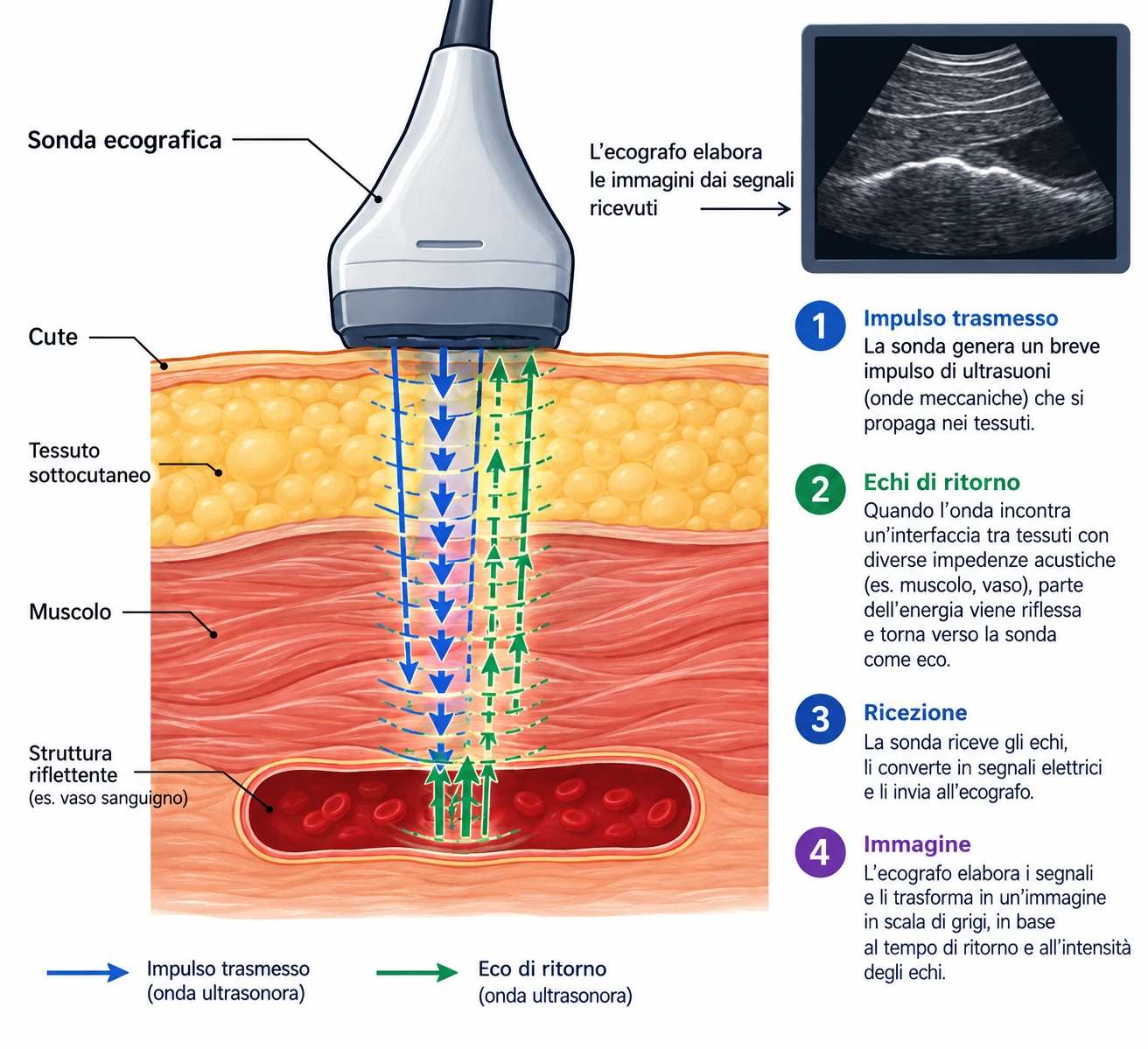
Diagnostic ultrasound uses mechanical waves with frequencies between about 2 and 15 MHz, generated and received by the same probe through piezoelectric crystals. The basic mechanism is simple: the probe emits a short pulse and then listens for the echo. From the time the echo takes to return, the scanner calculates the depth of the structure that reflected it.

L' amplitude of the returning echo depends on the difference in acoustic impedance between the tissues crossed by the ultrasound beam. The impedance difference between blood and vessel wall is small. Blood does not reflect like a mirror: red blood cells scatter a tiny fraction of the energy in all directions, and it is precisely this weak signal that Doppler analyses. Other tissues, such as bone and air, block the beam almost completely (hence the complete shadow behind bone and the impossibility of seeing through bowel gas).

Diagram of ultrasound image formation: the probe emits an ultrasound pulse that crosses skin, subcutaneous tissue and muscle; at the interface with a vessel part of the energy is reflected and returns to the probe as an echo; the probe converts the echoes into electrical signals and the scanner turns them into a greyscale image. Labels in Italian. — The cycle that generates the image: transmitted pulse, reflection at the interface between tissues with different acoustic impedance, reception of the echo and conversion to greyscale according to return time (depth) and echo strength (pixel brightness). *Tap the image to open it at full resolution (labels in Italian).*

Frequency, penetration, resolution

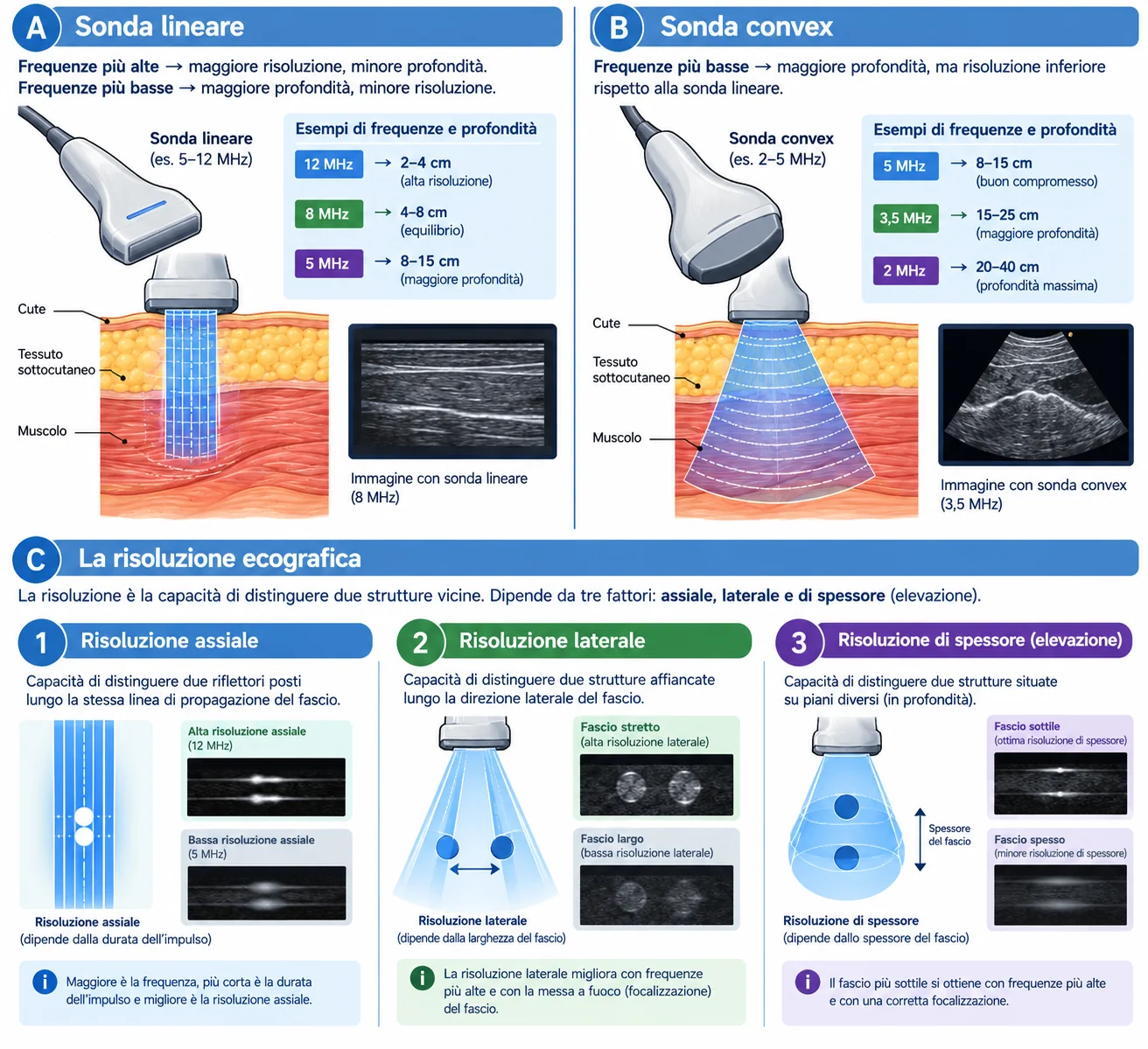
Attenuation of the ultrasound beam in soft tissue increases with frequency (roughly 0.5 dB per centimetre per MHz one way, i.e. about 1 dB/cm/MHz for the round trip): to image deep tissue well you therefore need a lower-frequency probe, while a higher frequency gives better resolution. This trade-off guides the choice of probe (e.g. a 3.5–5 MHz convex probe for greater penetration, a 12 MHz linear probe for better superficial resolution).

Axial resolution (along the beam direction): depends on pulse length, so it improves with frequency. It is the best of the three resolutions, which is why thickness measurements — IMT, plaque thickness, diameter — should be made with the interfaces perpendicular to the beam.
Lateral resolution (perpendicular to the beam, in the image plane): depends on beam width, and therefore on the focus. A badly placed focus widens the beam exactly where detail is needed.
Slice-thickness resolution (out of plane): the worst of the three, and it explains why a small eccentric plaque can "disappear" or look larger depending on probe tilt.

Choice of probe

Linear 5–12 MHz — carotid and vertebral arteries, upper and lower limbs, arteriovenous fistulas, superficial veins. Parallel beam, rectangular image, excellent resolution but limited penetration (roughly 4–6 cm).
High-frequency linear 9–18 MHz — very superficial vessels: distal calf arteries, dorsalis pedis, saphenous veins in thin subcutaneous tissue, pre-fistula mapping.
Convex 2–5 MHz — aorta and iliac arteries, renal and visceral arteries, vena cava, obese patients, deep vessels such as the external iliac or the distal deep femoral artery. Sector image, high penetration, lower resolution.
Microconvex or phased array — narrow acoustic windows: supraclavicular region, retroclavicular subclavian artery, intercostal spaces.

Comparison chart: 5–12 MHz linear probe with parallel beam and rectangular image, 2–5 MHz convex probe with diverging beam and sector image, examples of frequency and achievable depth, and the three types of ultrasound resolution — axial, lateral and slice-thickness (elevation). Labels in Italian. — On the left the linear probe and on the right the convex probe, with the order of magnitude of the depth that can be explored at each frequency; below, the three types of resolution: **axial** (depends on pulse duration, improves with frequency), **lateral** (depends on beam width, and therefore on the focus) and **slice-thickness** or elevation (depends on the out-of-plane thickness of the beam, and is the worst of the three). *Tap the image to open it at full resolution (labels in Italian).*

Tissue harmonics and compounding Tissue harmonic imaging (THI) clearly improves the signal-to-noise ratio in the abdomen and in difficult patients, reducing reverberation and side-lobe artefacts. Spatial compounding (an image built from several viewing angles) sharpens outlines but tends to soften posterior acoustic shadowing: if you need to recognise calcification or assess the shadow of a plaque, it is worth switching it off temporarily.

The Doppler effect and the angle of insonation

When the beam meets moving red blood cells, the echo returns at a frequency different from the one emitted. This difference — the Doppler shift — is proportional to blood velocity, but only to its component along the beam direction.

Δf = (2 · f₀ · v · cos θ) / c → v = (Δf · c) / (2 · f₀ · cos θ) Δf = Doppler shift · f₀ = transmitted frequency · v = blood velocity · θ = angle between beam and flow axis · c = 1540 m/s

The decisive term is cos θ. At 90° the cosine is zero: flow perpendicular to the beam produces no frequency shift, however fast it is. And it is close to 90° that the cosine changes most rapidly, i.e. where a small error in cursor alignment translates into a large velocity error.

With a linear probe the beam leaves perpendicular to the skin: on a vessel running parallel to the surface the angle is 90° and there is no Doppler signal. Tilting the probe (or steering the beam electronically) brings the angle down to 60° or less, and the velocity component along the beam becomes measurable.

Angle θ	cos θ	Velocity error for a ±5° misalignment
0°	1.00	negligible (< 1%)
45°	0.71	about ±8–10%
60°	0.50	about ±13–18%
70°	0.34	about ±20–30%
80°	0.17	from −33% to +100%
90°	0.00	measurement impossible

The three rules of the angle 1. Never exceed 60°: all published velocity thresholds — carotid, limb, renal — were derived with angles ≤ 60°, and above this value the numbers are no longer comparable with the literature.
2. The angle cursor must be aligned with the direction of flow, not with the wall and not with the box: in a stenosis the jet is oblique to the vessel axis, and colour shows where it points.
3. Always use the same angle at follow-up examinations of the same patient: much of the difference between one examination and the next arises here, not from the disease.

Pulsed-wave, continuous-wave Doppler and the Nyquist limit

Pulsed-wave Doppler (PW) samples at regular intervals, with a pulse repetition frequency (PRF) limited by depth: it can therefore tell where the signal comes from, but it cannot correctly display frequencies above half the PRF (the Nyquist limit). Above that thresholdaliasingappears: systolic peaks are "cut off" and wrap around to the opposite side of the baseline.

Continuous-wave Doppler (CW), available on some dedicated probes, has no Nyquist limit and measures very high velocities, but it adds up everything it meets along the beam line, without localisation. It is the choice when velocity exceeds what PW can measure.

What to do when aliasing appears Increase the scale (PRF); move the baseline down to dedicate the whole display to flow towards the probe; reduce image depth, which automatically raises the PRF; choose a lower transmit frequency (or the convex probe); increase the angle of insonation — within 60° — which reduces the shift; as a last resort, switch to continuous-wave Doppler.

Optimising the B-mode image

Colour and spectrum are built on the underlying image: if B-mode is badly set, everything else will be too. The order in which you adjust the scanner is always the same.

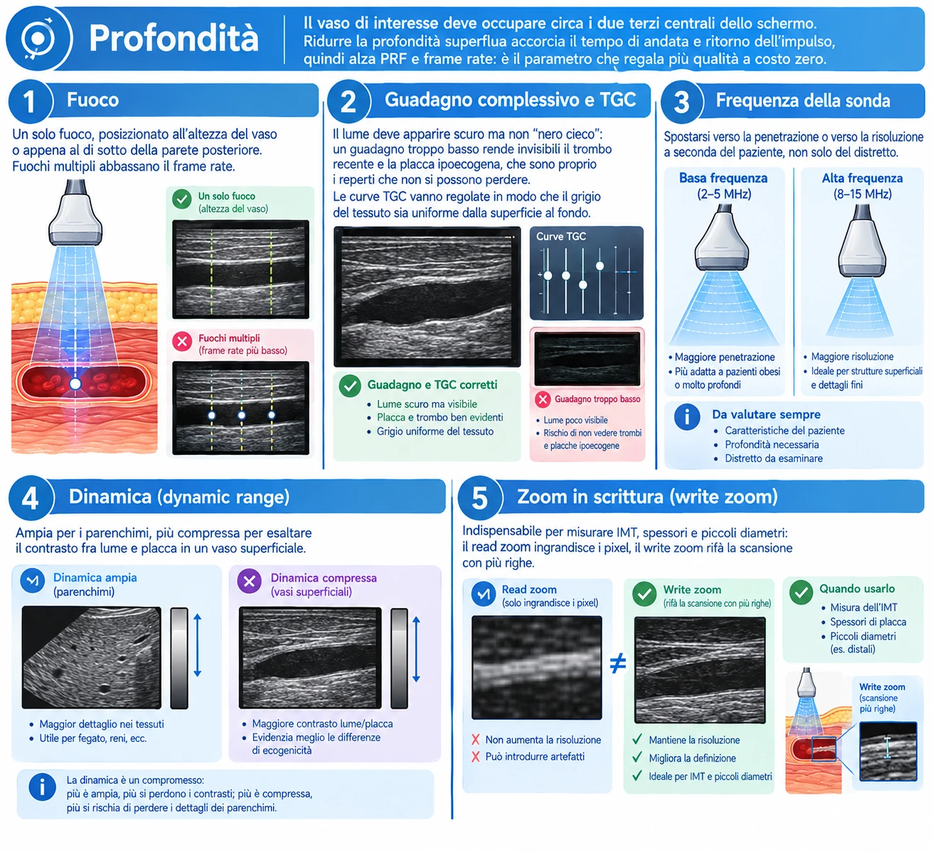
Depth — the vessel of interest should occupy roughly the central two thirds of the screen. Removing unnecessary depth shortens the pulse round-trip time, raising PRF and frame rate: it is the parameter that gives the most quality at no cost.
Focus — a single focal zone, placed at the level of the vessel or just below the far wall. Multiple focal zones lower the frame rate.
Overall gain and TGC — the lumen should look dark but not "blind black": too little gain makes fresh thrombus and hypoechoic plaque invisible, and these are exactly the findings that must not be missed. TGC curves should be adjusted so that tissue grey is uniform from the surface to the bottom.
Probe frequency — move towards penetration or towards resolution according to the patient, not only the territory.
Dynamic range — wide for parenchyma, more compressed to enhance contrast between lumen and plaque in a superficial vessel.
Write zoom (write zoom, not read zoom) — essential for measuring IMT, wall thickness and small diameters: read zoom enlarges the pixels, write zoom rescans with more lines.

Summary diagram of the parameters for optimising the B-mode image: vessel depth, single focus, overall gain and TGC curves, probe frequency (low or high), dynamic range and write zoom versus read zoom. Labels in Italian. — The controls to adjust, in order: depth, focus, gain and TGC, probe frequency, dynamic range and write zoom. *Tap the image to open it at full resolution (labels in Italian).*

Probe pressure Contact should be light and gel plentiful. Excessive pressure compresses veins — simulating thrombosis, abolishing reflux — and can squash superficial arteries, creating a local acceleration that resembles a stenosis. It is a common mistake made precisely when trying to "see better".

The colour box: position, size, steering

Colour Doppler encodes in a colour map the mean Doppler shift of each small volume inside the box. Colour indicates direction relative to the probe — towards or away from it — and not the nature of the vessel: red does not mean artery, blue does not mean vein.

With a linear probe, electronic steering of the box is the quickest way to get away from 90° without losing the anatomic plane. Steer it towards the side the flow comes from, and switch it off when the vessel is already oblique to the skin surface.

Size and position

Keep the box as small as possible, just wider than the vessel. Every extra line of colour costs time: a box twice as wide halves the frame rate, and with it the ability to capture rapid events (systolic jet, brief reflux).
The depth of the box should be limited to the vessel: colour over tissue of no interest means only noise and slowness.
With a convex probe the beam diverges: in the centre of the sector a horizontal vessel is at 90°, at the edges it is not. Simply moving the vessel to the side of the image often gives a useful angle without changing any setting.

Steering

Electronic steering of the box, typically by 15–25°, moves the beam without moving the probe. It has a cost: a steered beam uses a smaller portion of the array and sensitivity falls, the more so the greater the steering. Use it when needed and return it to zero when the vessel is already oblique — for example at the carotid bulb, in the calf arteries or along a deep femoral axis.

Box steering and the angle cursor are two different things Steering the box changes the physical direction of the beam; the angle cursor only tells the scanner how to correct the calculation. Steering the box without realigning the cursor, or vice versa, produces wrong velocities even when the image looks correct.

The controls that matter

Parameter	If too low	If too high
Colour scale / PRF	Widespread aliasing, colour mosaic in a normal vessel, overestimated velocity	Slow flow invisible: patent vein mistaken for thrombosed, near-occlusion mistaken for occlusion
Colour gain	Incomplete lumen, false filling defects, overestimated plaque	Colour spilling beyond the wall (blooming), stenosis masked
Wall filter	Wall and tissue motion artefacts	Removes slow diastolic and venous flow
Persistence	Noisy, "jittery" image	Artificial filling, rapid events averaged out and unrecognisable
Colour / B-mode priority	Colour does not appear over light grey tones	Colour covers hypoechoic plaque and leads to underestimation of the stenosis

Quick method for colour gain Increase the gain until colour speckles appear in the tissue around the vessel, then reduce it slightly until they disappear: this is the point of maximum sensitivity without noise. Repeat whenever you change depth, frequency or territory.

The sample volume and the pulsed-wave Doppler spectrum

Colour locates and orients; measurement is done with pulsed-wave Doppler. The sample volume (gate) defines which portion of the lumen the spectrum comes from, and its size should be chosen according to what you want to measure.

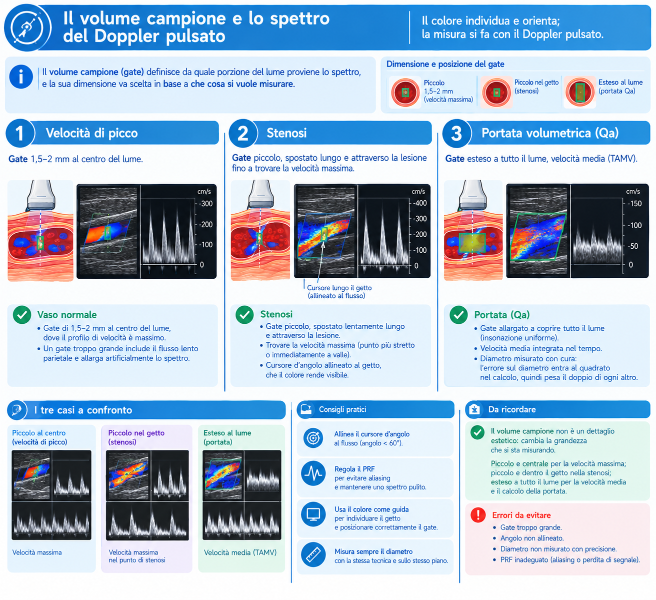
Normal vessel — a 1.5–2 mm gate in the centre of the lumen, where the velocity profile is highest. Too large a gate includes slow flow near the wall and artificially broadens the spectrum.
Stenosis — small gate, moved slowly along and across the lesion until the peak velocity is found, at the narrowest point or immediately beyond it. Align the angle cursor with the jet, which colour makes visible.
Volume flow — gate opened to cover the whole lumen (uniform insonation), time-averaged mean velocity and a carefully measured diameter: the diameter error is squared in the calculation, so it weighs twice as much as any other.

Spectral settings

Scale and baseline — the spectrum should fill two thirds of the display without aliasing and without being squashed against the baseline.
PW gain — enough for a full trace with a sharp outline, but not so much that noise fills the spectral window under the curve.
Wall filter — low (50–100 Hz) for venous studies and slow diastolic flow; a high filter removes diastolic flow and can lead to a mistaken diagnosis of distal occlusion or increased resistance.
Sweep speed — 50–100 mm/s for analysing waveform shape (acceleration time, tardus-parvus); slower for dynamic manoeuvres, which need several seconds of trace: Valsalva, calf squeeze, reactive hyperaemia.

The spectral window In laminar flow the area under the curve stays dark: all the red cells travel at similar velocities. Filling of the window (spectral broadening) indicates turbulence, but an oversized gate, excessive gain or sampling too close to the wall also fill it in the absence of any disease. Before reporting turbulence, it is worth resampling with a small gate and correct gain.

Power Doppler and other modes

Power Doppler maps the amplitude of the Doppler signal instead of its mean frequency. It loses direction and velocity information but gains sensitivity to slow flow, is practically angle-independent and is not subject to aliasing. It is the mode to use when the question is "is there flow or not?": distinguishing occlusion from near-occlusion with trickle flow, looking for recanalisation in a vein, intraparenchymal renal vessels, residual flow inside a partially thrombosed aneurysm. On the other hand it is very sensitive to motion: a single breath can fill the screen with colour (flash artefact), and high persistence makes it unsuitable for assessing temporal dynamics.

The microvascular imaging modes on recent machines (with different names from one manufacturer to another) and B-flow filter tissue motion more selectively and show slow flow with better spatial resolution: useful for the residual lumen of a plaque and for small vessels. Contrast-enhanced ultrasound has defined vascular indications — above all the search for endoleak after endovascular aneurysm repair — but is beyond the scope of the basic examination.

Presets and settings by territory

Every scanner leaves the factory with reasonable vascular presets: the useful work is to refine them once and save them, so that every examination starts from a known point rather than from the settings left by the previous patient. The values below are indicative and must be adapted to the patient and the machine.

Territory	Probe	Colour scale	Wall filter and practical notes
Supra-aortic trunks	Linear 5–12 MHz	25–40 cm/s (higher across stenoses)	Medium filter. Box steered over the common carotid, steering at zero at the bulb; a constant 60° angle, stated in the report
Lower-limb arteries	Linear 4–9 MHz; convex 2–5 MHz for iliac arteries and obese patients	30–50 cm/s	Medium-high filter. Reduce the scale in segments beyond an occlusion, where flow is slow and damped
Calf arteries and dorsalis pedis	Linear 9–15 MHz	10–20 cm/s	Low filter. Very light contact and plenty of gel: flow may be barely detectable
Lower-limb veins	Linear 5–9 MHz; convex for iliac veins and vena cava	8–15 cm/s	Low filter, high persistence, generous colour gain; compression always in transverse view
Abdominal arteries	Convex 2–5 MHz with harmonics	30–50 cm/s	Medium filter. 6–8 hours of fasting, brief breath-hold for sampling, deep focus
Renal arteries	Convex 2–5 MHz	30–40 cm/s (lower for intraparenchymal vessels)	Low filter inside the kidney. Small box and reproducible breath-hold; power Doppler useful for segmental vessels
Arteriovenous fistula	Linear 5–12 MHz (convex if the access is deep)	60–100 cm/s and above	Medium-high filter. Velocities in a mature access far exceed native ones: very high scale and wide gate for volume flow
Upper limbs	Linear 5–12 MHz	20–40 cm/s (arterial), 8–15 cm/s (venous)	Low filter for veins. Microconvex for the retroclavicular subclavian; positional manoeuvres for thoracic outlet

What is really worth saving in a preset Starting depth and focus, probe frequency, dynamic range, colour map and its scale, wall filter, persistence, default gate size, spectral sweep speed and display format (image only, image + spectrum, triplex). The rest is adjusted to the patient. It is worth having separate arterial and venous presets for the same territory: they differ mainly in scale and filter, i.e. the two parameters that cause the most serious errors.

Longitudinal and transverse scanning

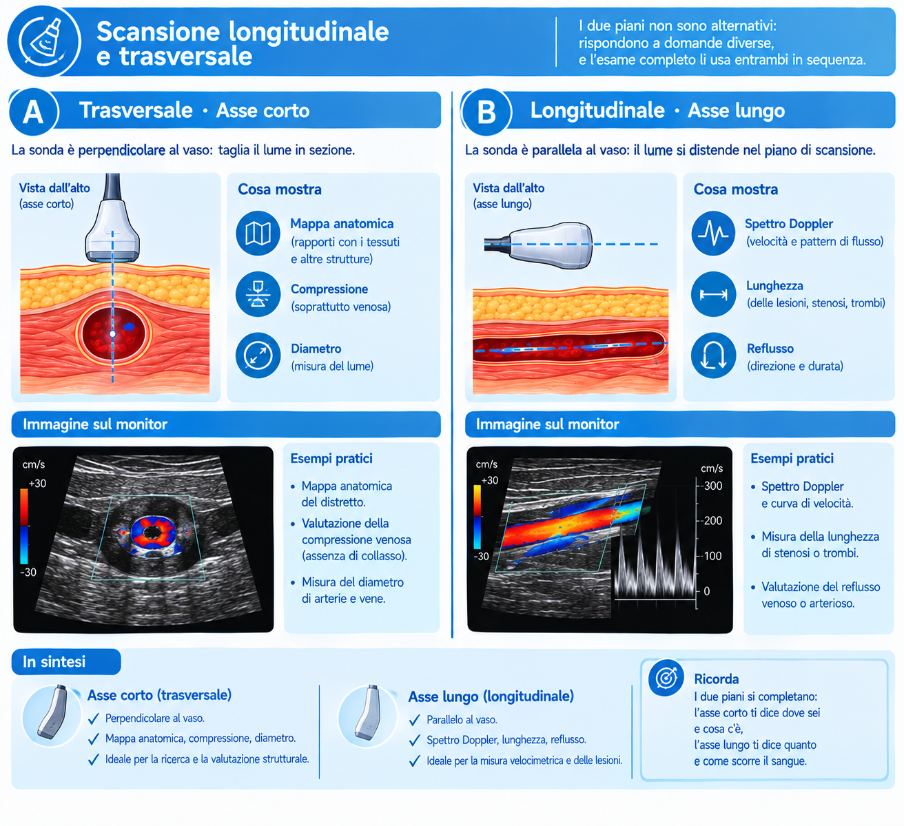
The two planes are not alternatives: they answer different questions, and a complete examination uses both in sequence.

When the transverse view is needed

Surveying the vessel from start to finish with colour on: the quickest and safest way not to skip a segment. A diseased segment "jumps out" as a filling defect or colour mosaic.
Venous compression: performed exclusively in transverse view. In the longitudinal view the vein slips out of the scan plane and appears compressible even when it contains thrombus.
Diameter of the aorta and aneurysms: the measurement must be taken perpendicular to the vessel axis. In a tortuous aorta an oblique section overestimates the calibre, and it is the most common cause of aneurysms that have apparently "grown" between two checks without really doing so.
Circumferential extent of plaque and its eccentricity, which are poorly assessed in the long axis.

When the longitudinal view is needed

Doppler spectrum with correct angle: it is the only plane in which the flow axis can be identified and the cursor reliably aligned.
Length of the stenosis or occlusion, distance from the origin and relationship with the bifurcation: data the surgeon or interventionist uses for planning.
IMT and wall thickness, exploiting axial resolution on the far wall.
Venous reflux and dynamic manoeuvres, where a continuous spectral trace is needed.

The vessel cut obliquely An oblique section is the trap of both planes: in transverse view it makes the lumen elliptical and simulates a reduction in calibre; in longitudinal view it shows non-parallel walls and overestimates the diameter. The practical rule is to look, with small rotations of the probe, for the plane in which the vessel appears smallest and roundestin the short axis and widest, with parallel, well-defined wallsin the long axis: that is the true plane.

Recommended sequence Survey the territory in transverse view with colour, identifying suspicious points; return in longitudinal view to each of them for spectral quantification; finish with the dynamic manoeuvres for that territory. Document at least one image per segment and one spectrum for each significant finding: what has not been measured cannot be described in the report.

Recurrent artefacts and pitfalls

Artefact	How to recognise it	What to do
Aliasing	Colour mosaic in the lumen, spectral peaks cut off and wrapped to the opposite side	Raise the scale, lower the baseline, reduce depth, increase the angle within 60°
90° angle	No colour, or colour change in the middle of a curved vessel, with a normal lumen on B-mode	Steer the box or tilt the probe; never report as stenosis or occlusion
Acoustic shadowing from calcification	Anechoic cone behind the plaque, colour and spectrum unobtainable	Change window and plane; if it persists, state the limitation in the report and rely on the waveform downstream
Mirror image	Vessel or spectrum "duplicated" beyond a strong interface (pleura, clavicle, diaphragm)	Recognise the symmetry about the interface; change the angle of approach
Blooming / colour bleeding	Colour overflows beyond the wall and covers the plaque	Reduce colour gain and colour priority; compare with B-mode without colour
Twinkling	Colour scintillation behind a calcified structure	Recognise it as an artefact; sometimes useful for detecting calcification
Reverberation in the lumen	Linear echoes in the lumen of a superficial vessel, resembling thrombus	Change angle and depth; check with colour and power Doppler
Flash artefact	Sudden, diffuse filling with colour on breathing or movement	Brief breath-hold, lower persistence, higher wall filter
False absence of flow	"Empty" vessel with high PRF, high filter or low gain	Before writing occlusion: lower the scale, lower the filter, raise the gain, try power Doppler

The rule that prevents the most serious errors No diagnosis of occlusion should be made with a single machine setting. Absence of flow is the conclusion that most easily arises from a badly set scanner, and it has immediate clinical consequences: before stating it, high PRF, high wall filter, insufficient gain and an angle close to 90° must be excluded.

Safety and the ALARA principle

Diagnostic ultrasound does not use ionising radiation, but it deposits mechanical and thermal energy. The display shows two indices: themechanical index (MI), related to the risk of cavitation, and thethermal index (TI), which estimates tissue heating — with variants for soft tissue, bone and cranial bone.

Pulsed-wave and colour Doppler concentrate much more energy than B-mode, because they insonate the same line repeatedly. The ALARA (as low as reasonably achievable) principle therefore applies: keep acoustic output at the lowest useful level and raise receive gain instead, limit the duration of Doppler insonation at the same site, and take particular care in pregnancy and in children. In adult vascular patients the margins are wide, but good habits cost nothing.

Hygiene and the probe Disinfect the probe between patients according to the manufacturer's protocol, avoid incompatible solutions that damage the acoustic lens, and use a sterile cover when the examination guides a procedure (ultrasound-guided puncture, pre-operative mapping with skin marking).

Sources

Hoskins PR, Martin K, Thrush A (eds), CRC Press 2019 — Diagnostic Ultrasound: Physics and Equipment, 3rd edition. Image formation, attenuation, Doppler principles, artefacts and safety.
Kremkau FW, Elsevier 2021 — Sonography Principles and Instruments, 10th edition. Ultrasound physics, instrumentation, Doppler and bioeffects.
Thrush A, Hartshorne T, Deane CR, Elsevier 2022 — Vascular Ultrasound: How, Why and When, 4th edition. Application to vascular scanning: angle of insonation, colour and pulsed-wave Doppler settings, artefacts.

The values in the angle-error table are calculated from the Doppler equation (the estimated velocity is inversely proportional to the cosine of the angle) for a ±5° misalignment from the set angle.

Physical principles and ultrasound machine settings